7.6 KiB
Recurrent Neural Networks
Pre-lecture quiz
In previous sections, we used rich semantic representations of text combined with a simple linear classifier on top of embeddings. This architecture captures the overall meaning of words in a sentence but does not account for the order of words, as the aggregation operation on embeddings removes this information from the original text. Since these models cannot model word order, they struggle with more complex or ambiguous tasks like text generation or question answering.
To understand the meaning of text sequences, we need a different neural network architecture called a recurrent neural network (RNN). In an RNN, we process a sentence one symbol at a time through the network, which produces a state that is then passed back into the network along with the next symbol.

Image by the author
Given an input sequence of tokens X0,...,Xn, an RNN creates a sequence of neural network blocks and trains this sequence end-to-end using backpropagation. Each network block takes a pair (Xi,Si) as input and produces Si+1 as output. The final state Sn (or output Yn) is passed to a linear classifier to generate the result. All network blocks share the same weights and are trained end-to-end in a single backpropagation pass.
Because the state vectors S0,...,Sn are passed through the network, it can learn sequential dependencies between words. For instance, when the word not appears in the sequence, the network can learn to negate certain elements within the state vector, enabling negation.
✅ Since the weights of all RNN blocks in the image above are shared, the same structure can be represented as a single block (on the right) with a recurrent feedback loop that passes the network's output state back to the input.
Anatomy of an RNN Cell
Let’s explore the structure of a simple RNN cell. It takes the previous state Si-1 and the current symbol Xi as inputs and produces the output state Si. Sometimes, we are also interested in another output Yi, as in generative networks.
A simple RNN cell contains two weight matrices: one transforms the input symbol (let’s call it W), and the other transforms the input state (H). The network output is calculated as σ(W×Xi+H×Si-1+b), where σ is the activation function and b is an additional bias.

Image by the author
In many cases, input tokens are passed through an embedding layer before entering the RNN to reduce dimensionality. If the input vector dimension is emb_size and the state vector dimension is hid_size, the size of W is emb_size×hid_size, and the size of H is hid_size×hid_size.
Long Short Term Memory (LSTM)
One major issue with classical RNNs is the vanishing gradients problem. Since RNNs are trained end-to-end in a single backpropagation pass, it becomes difficult to propagate errors to the earlier layers of the network, preventing the network from learning relationships between distant tokens. One solution to this problem is explicit state management using gates. Two popular architectures that implement this are Long Short Term Memory (LSTM) and Gated Relay Unit (GRU).
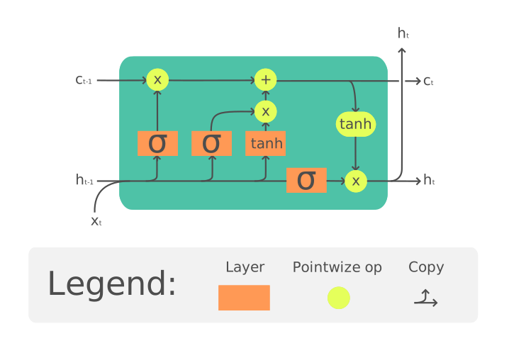
Image source TBD
The LSTM network is similar to an RNN but passes two states between layers: the actual state C and the hidden vector H. At each unit, the hidden vector Hi is concatenated with the input Xi, and together they control the state C via gates. Each gate is a neural network with sigmoid activation (output range [0,1]), which acts like a bitwise mask when multiplied by the state vector. The gates (from left to right in the image above) are:
- The forget gate determines which components of the vector C should be forgotten and which should be retained.
- The input gate extracts information from the input and hidden vectors and inserts it into the state.
- The output gate transforms the state via a linear layer with tanh activation and selects certain components using the hidden vector Hi to produce a new state Ci+1.
The components of state C can be thought of as flags that can be toggled on or off. For example, encountering the name Alice in a sequence might raise a flag indicating a female noun. Later, encountering the phrase and Tom might raise a flag indicating a plural noun. By manipulating the state, the network can track grammatical properties of sentence parts.
✅ A great resource for understanding LSTM internals is Christopher Olah’s article Understanding LSTM Networks.
Bidirectional and Multilayer RNNs
So far, we’ve discussed recurrent networks that process sequences in one direction, from start to finish. This approach feels natural since it mimics how we read or listen to speech. However, in many practical scenarios, we have random access to the input sequence, making it useful to run recurrent computations in both directions. Such networks are called bidirectional RNNs. In bidirectional networks, two hidden state vectors are maintained—one for each direction.
A recurrent network, whether unidirectional or bidirectional, captures patterns within a sequence and stores them in a state vector or passes them to the output. Similar to convolutional networks, we can stack another recurrent layer on top of the first to capture higher-level patterns based on the low-level patterns extracted by the first layer. This leads to the concept of a multi-layer RNN, which consists of two or more recurrent networks, where the output of one layer serves as the input to the next.

Picture from this wonderful post by Fernando López
✍️ Exercises: Embeddings
Continue your learning in the following notebooks:
Conclusion
In this unit, we’ve seen that RNNs can be used for sequence classification, but they are capable of much more, including tasks like text generation, machine translation, and more. We’ll explore these tasks in the next unit.
🚀 Challenge
Read some literature about LSTMs and explore their applications:
- Grid Long Short-Term Memory
- Show, Attend and Tell: Neural Image Caption Generation with Visual Attention
Post-lecture quiz
Review & Self Study
- Understanding LSTM Networks by Christopher Olah.