AI-For-Beginners/etc/docsify-to-pdf/static/main.md

Introduction to AI

Sketchnote by Tomomi Imura

Pre-lecture quiz

Artificial Intelligence is an exciting scientific discipline that studies how we can make computers exhibit intelligent behavior, e.g. do those things that human beings are good at doing.

Originally, computers were invented by Charles Babbage to operate on numbers following a well-defined procedure - an algorithm. Modern computers, even though significantly more advanced than the original model proposed in the 19th century, still follow the same idea of controlled computations. Thus it is possible to program a computer to do something if we know the exact sequence of steps that we need to do in order to achieve the goal.

Photo by Vickie Soshnikova

✅ Defining the age of a person from his or her photograph is a task that cannot be explicitly programmed, because we do not know how we come up with a number inside our head when we do it.

---

There are some tasks, however, that we do not explicitly know how to solve. Consider determining the age of a person from his/her photograph. We somehow learn to do it, because we have seen many examples of people of different age, but we cannot explicitly explain how we do it, nor can we program the computer to do it. This is exactly the kind of task that are of interest to Artificial Intelligence (AI for short).

✅ Think of some tasks that you could offload to a computer that would benefit from AI. Consider the fields of finance, medicine, and the arts - how are these fields benefiting today from AI?

Weak AI vs. Strong AI

The task of solving a specific human-like problem, such as determining a person's age from a photo, can be called Weak AI, because we are creating a system for only one task, and not a system that can solve many tasks, such as can be done by a human being. Of course, developing a generally intelligent computer system is also extremely interesting from many points of view, including for students of the philosophy of consciousness. Such system would be called Strong AI, or Artificial General Intelligence (AGI).

The Definition of Intelligence and the Turing Test

One of the problems when dealing with the term Intelligence is that there is no clear definition of this term. One can argue that intelligence is connected to abstract thinking, or to self-awareness, but we cannot properly define it.

Photo by Amber Kipp from Unsplash

To see the ambiguity of a term intelligence, try answering a question: "Is a cat intelligent?". Different people tend to give different answers to this question, as there is no universally accepted test to prove the assertion true or not. And if you think there is - try running your cat through an IQ test...

✅ Think for a minute about how you define intelligence. Is a crow who can solve a maze and get at some food intelligent? Is a child intelligent?

---

When speaking about AGI we need to have some way to tell if we have created a truly intelligent system. Alan Turing proposed a way called a Turing Test, which also acts like a definition of intelligence. The test compares a given system to something inherently intelligent - a real human being, and because any automatic comparison can be bypassed by a computer program, we use a human interrogator. So, if a human being is unable to distinguish between a real person and a computer system in text-based dialogue - the system is considered intelligent.

A chat-bot called Eugene Goostman, developed in St.Petersburg, came close to passing the Turing test in 2014 by using a clever personality trick. It announced up front that it was a 13-year old Ukrainian boy, which would explain the lack of knowledge and some discrepancies in the text. The bot convinced 30% of the judges that it was human after a 5 minute dialogue, a metric that Turing believed a machine would be able to pass by 2000. However, one should understand that this does not indicate that we have created an intelligent system, or that a computer system has fooled the human interrogator - the system didn't fool the humans, but rather the bot creators did!

✅ Have you ever been fooled by a chat bot into thinking that you are speaking to a human? How did it convince you?

Different Approaches to AI

If we want a computer to behave like a human, we need somehow to model inside a computer our way of thinking. Consequently, we need to try to understand what makes a human being intelligent.

To be able to program intelligence into a machine, we need to understand how our own processes of making decisions work. If you do a little self-introspection, you will realize that there are some processes that happen subconsciously – eg. we can distinguish a cat from a dog without thinking about it - while some others involve reasoning.

There are two possible approaches to this problem:

Top-down Approach (Symbolic Reasoning)	Bottom-up Approach (Neural Networks)
A top-down approach models the way a person reasons to solve a problem. It involves extracting knowledge from a human being, and representing it in a computer-readable form. We also need to develop a way to model reasoning inside a computer.	A bottom-up approach models the structure of a human brain, consisting of huge number of simple units called neurons. Each neuron acts like a weighted average of its inputs, and we can train a network of neurons to solve useful problems by providing training data.

There are also some other possible approaches to intelligence:

• An Emergent, Synergetic or multi-agent approach are based on the fact that complex intelligent behaviour can be obtained by an interaction of a large number of simple agents. According to evolutionary cybernetics, intelligence can emerge from more simple, reactive behaviour in the process of metasystem transition.

• An Evolutionary approach, or genetic algorithm is an optimization process based on the principles of evolution.

We will consider those approaches later in the course, but right now we will focus on two main directions: top-down and bottom-up.

The Top-Down Approach

In a top-down approach, we try to model our reasoning. Because we can follow our thoughts when we reason, we can try to formalize this process and program it inside the computer. This is called symbolic reasoning.

People tend to have some rules in their head that guide their decision making processes. For example, when a doctor is diagnosing a patient, he or she may realize that a person has a fever, and thus there might be some inflammation going on inside the body. By applying a large set of rules to a specific problem a doctor may be able to come up with the final diagnosis.

This approach relies heavily on knowledge representation and reasoning. Extracting knowledge from a human expert might be the most difficult part, because a doctor in many cases would not know exactly why he or she is coming up with a particular diagnosis. Sometimes the solution just comes up in his or her head without explicit thinking. Some tasks, such as determining the age of a person from a photograph, cannot be at all reduced to manipulating knowledge.

Bottom-Up Approach

Alternately, we can try to model the simplest elements inside our brain – a neuron. We can construct a so-called artificial neural network inside a computer, and then try to teach it to solve problems by giving it examples. This process is similar to how a newborn child learns about his or her surroundings by making observations.

✅ Do a little research on how babies learn. What are the basic elements of a baby's brain?

What about ML?
Part of Artificial Intelligence that is based on computer learning to solve a problem based on some data is called Machine Learning. We will not consider classical machine learning in this course - we refer you to a separate Machine Learning for Beginners curriculum.

A Brief History of AI

Artificial Intelligence was started as a field in the middle of the twentieth century. Initially symbolic reasoning was a prevalent approach, and it led to a number of important successes, such as expert systems – computer programs that were able to act as an expert in some limited problem domain. However, it soon became clear that such approach does not scale well. Extracting the knowledge from an expert, representing it in a computer, and keeping that knowledgebase accurate turns out to be a very complex task, and too expensive to be practical in many cases. This led to so-called AI Winter in the 1970s.

Image by Dmitry Soshnikov

As time passed, computing resources became cheaper, and more data has become available, so neural network approaches started demonstrating great performance in competing with human beings in many areas, such as computer vision or speech understanding. In the last decade, the term Artificial Intelligence has been mostly used as a synonym for Neural Networks, because most of the AI successes that we hear about are based on them.

We can observe how the approaches changed, for example, in creating a chess playing computer program:

• Early chess programs were based on search – a program explicitly tried to estimate possible moves of an opponent for a given number of next moves, and selected an optimal move based on the optimal position that can be achieved in a few moves. It led to the development of the so-called alpha-beta pruning search algorithm.
• Search strategies work well towards the end of the game, where the search space is limited by a small number of possible moves. However, in the beginning of the game the search space is huge, and the algorithm can be improved by learning from existing matches between human players. Subsequent experiments employed so-called case-based reasoning, where the program looked for cases in the knowledge base very similar to the current position in the game.
• Modern programs that win over human players are based on neural networks and reinforcement learning, where the programs learn to play solely by playing a long time against itself and learning from its own mistakes – much like human beings do when learning to play chess. However, a computer program can play many more games in much less time, and thus can learn much faster.

✅ Do a little research on other games that have been played by AI.

Similarly, we can see how the approach towards creating “talking programs” (that might pass the Turing test) changed:

• Early programs of this kind such as Eliza, were based on very simple grammatical rules and the re-formulation of the input sentence into a question.
• Modern assistants, such as Cortana, Siri or Google Assistant are all hybrid systems that use Neural networks to convert speech into text and to recognize our intent, and then employ some reasoning or explicit algorithms to perform required actions.
• In the future, we may expect complete neural-based model to handle dialogue by itself. The recent GPT and Turing-NLG family of neural networks show great success in this.

Image by Dmitry Soshnikov, photo by Marina Abrosimova, Unsplash

Recent AI Research

The huge recent growth in neural network research started around 2010, when large public datasets started to become available. A huge collection of images called ImageNet, which contains around 14 million annotated images, gave birth to the ImageNet Large Scale Visual Recognition Challenge.

Image by Dmitry Soshnikov

In 2012, Convolutional Neural Networks were first used in image classification, which led to a significant drop in classification errors (from almost 30% to 16.4%). In 2015, ResNet architecture from Microsoft Research achieved human-level accuracy.

Since then, Neural Networks demonstrated very successful behaviour in many tasks:

---

Year	Human Parity achieved
2015	Image Classification
2016	Conversational Speech Recognition
2018	Automatic Machine Translation (Chinese-to-English)
2020	Image Captioning

Over the past few years we have witnessed huge successes with large language models, such as BERT and GPT-3. This happen happened mostly due to the fact that there is a lot of general text data available that allows us to train models to capture the structure and meaning of texts, pre-train them on general text collections, and then specialize those models for more specific tasks. We will learn more about Natural Language Processing later in this course.

🚀 Challenge

Do a tour of the internet to determine where, in your opinion, AI is most effectively used. Is it in a Mapping app, or some speech-to-text service or a video game? Research how the system was built.

Post-lecture quiz

Review & Self Study

Review the history of AI and ML by reading through this lesson. Take an element from the sketchnote at the top of that lesson or this one and research it in more depth to understand the cultural context informing its evolution.

Assignment: Game Jam

Knowledge Representation and Expert Systems

Sketchnote by Tomomi Imura

The quest for artificial intelligence is based on a search for knowledge, to make sense of the world similar to how humans do. But how can you go about doing this?

Pre-lecture quiz

In the early days of AI, the top-down approach to creating intelligent systems (discussed in the previous lesson) was popular. The idea was to extract the knowledge from people into some machine-readable form, and then use it to automatically solve problems. This approach was based on two big ideas:

• Knowledge Representation
• Reasoning

Knowledge Representation

One of the important concepts in Symbolic AI is knowledge. It is important to differentiate knowledge from information or data. For example, one can say that books contain knowledge, because one can study books and become an expert. However, what books contain is actually called data, and by reading books and integrating this data into our world model we convert this data to knowledge.

✅ Knowledge is something which is contained in our head and represents our understanding of the world. It is obtained by an active learning process, which integrates pieces of information that we receive into our active model of the world.

Most often, we do not strictly define knowledge, but we align it with other related concepts using DIKW Pyramid. It contains the following concepts:

• Data is something represented in physical media, such as written text or spoken words. Data exists independently of human beings and can be passed between people.
• Information is how we interpret data in our head. For example, when we hear the word computer, we have some understanding of what it is.
• Knowledge is information being integrated into our world model. For example, once we learn what a computer is, we start having some ideas about how it works, how much it costs, and what it can be used for. This network of interrelated concepts forms our knowledge.
• Wisdom is yet one more level of our understanding of the world, and it represents meta-knowledge, eg. some notion on how and when the knowledge should be used.

Image from Wikipedia, By Longlivetheux - Own work, CC BY-SA 4.0

Thus, the problem of knowledge representation is to find some effective way to represent knowledge inside a computer in the form of data, to make it automatically usable. This can be seen as a spectrum:

Image by Dmitry Soshnikov

• On the left, there are very simple types of knowledge representations that can be effectively used by computers. The simplest one is algorithmic, when knowledge is represented by a computer program. This, however, is not the best way to represent knowledge, because it is not flexible. Knowledge inside our head is often non-algorithmic.
• On the right, there are representations such as natural text. It is the most powerful, but cannot be used for automatic reasoning.

✅ Think for a minute about how you represent knowledge in your head and convert it to notes. Is there a particular format that works well for you to aid in retention?

Classifying Computer Knowledge Representations

We can classify different computer knowledge representation methods in the following categories:

• Network representations are based on the fact that we have a network of interrelated concepts inside our head. We can try to reproduce the same networks as a graph inside a computer - a so-called semantic network.

1. Object-Attribute-Value triplets or attribute-value pairs. Since a graph can be represented inside a computer as a list of nodes and edges, we can represent a semantic network by a list of triplets, containing objects, attributes, and values. For example, we build the following triplets about programming languages:

Object	Attribute	Value
Python	is	Untyped-Language
Python	invented-by	Guido van Rossum
Python	block-syntax	indentation
Untyped-Language	doesn't have	type definitions

✅ Think how triplets can be used to represent other types of knowledge.

2. Hierarchical representations emphasize the fact that we often create a hierarchy of objects inside our head. For example, we know that canary is a bird, and all birds have wings. We also have some idea about what colour canary usually is, and what is their flight speed.

   • Frame representation is based on representing each object or class of objects as a frame which contains slots. Slots have possible default values, value restrictions, or stored procedures that can be called to obtain the value of a slot. All frames form a hierarchy similar to an object hierarchy in object-oriented programming languages.
   • Scenarios are special kind of frames that represent complex situations that can unfold in time.

Python

Slot	Value	Default value	Interval
Name	Python
Is-A	Untyped-Language
Variable Case		CamelCase
Program Length			5-5000 lines
Block Syntax	Indent

3. Procedural representations are based on representing knowledge by a list of actions that can be executed when a certain condition occurs.

   • Production rules are if-then statements that allow us to draw conclusions. For example, a doctor can have a rule saying that IF a patient has high fever OR high level of C-reactive protein in blood test THEN he has an inflammation. Once we encounter one of the conditions, we can make a conclusion about inflammation, and then use it in further reasoning.
   • Algorithms can be considered another form of procedural representation, although they are almost never used directly in knowledge-based systems.

4. Logic was originally proposed by Aristotle as a way to represent universal human knowledge.

   • Predicate Logic as a mathematical theory is too rich to be computable, therefore some subset of it is normally used, such as Horn clauses used in Prolog.
   • Descriptive Logic is a family of logical systems used to represent and reason about hierarchies of objects distributed knowledge representations such as semantic web.

Expert Systems

One of the early successes of symbolic AI were so-called expert systems - computer systems that were designed to act as an expert in some limited problem domain. They were based on a knowledge base extracted from one or more human experts, and they contained an inference engine that performed some reasoning on top of it.

Simplified structure of a human neural system	Architecture of a knowledge-based system

Expert systems are built like the human reasoning system, which contains short-term memory and long-term memory. Similarly, in knowledge-based systems we distinguish the following components:

• Problem memory: contains the knowledge about the problem being currently solved, i.e. the temperature or blood pressure of a patient, whether he has inflammation or not, etc. This knowledge is also called static knowledge, because it contains a snapshot of what we currently know about the problem - the so-called problem state.
• Knowledge base: represents long-term knowledge about a problem domain. It is extracted manually from human experts, and does not change from consultation to consultation. Because it allows us to navigate from one problem state to another, it is also called dynamic knowledge.
• Inference engine: orchestrates the whole process of searching in the problem state space, asking questions of the user when necessary. It is also responsible for finding the right rules to be applied to each state.

As an example, let's consider the following expert system of determining an animal based on its physical characteristics:

Image by Dmitry Soshnikov

This diagram is called an AND-OR tree, and it is a graphical representation of a set of production rules. Drawing a tree is useful at the beginning of extracting knowledge from the expert. To represent the knowledge inside the computer it is more convenient to use rules:

IF the animal eats meat
OR (animal has sharp teeth
    AND animal has claws
    AND animal has forward-looking eyes
) 
THEN the animal is a carnivore

You can notice that each condition on the left-hand-side of the rule and the action are essentially object-attribute-value (OAV) triplets. Working memory contains the set of OAV triplets that correspond to the problem currently being solved. A rules engine looks for rules for which a condition is satisfied and applies them, adding another triplet to the working memory.

✅ Write your own AND-OR tree on a topic you like!

Forward vs. Backward Inference

The process described above is called forward inference. It starts with some initial data about the problem available in the working memory, and then executes the following reasoning loop:

1. If the target attribute is present in the working memory - stop and give the result
2. Look for all the rules whose condition is currently satisfied - obtain conflict set of rules.
3. Perform conflict resolution - select one rule that will be executed on this step. There could be different conflict resolution strategies:
   • Select the first applicable rule in the knowledge base
   • Select a random rule
   • Select a more specific rule, i.e. the one meeting the most conditions in the "left-hand-side" (LHS)
4. Apply selected rule and insert new piece of knowledge into the problem state
5. Repeat from step 1.

However, in some cases we might want to start with an empty knowledge about the problem, and ask questions that will help us arrive to the conclusion. For example, when doing medical diagnosis, we usually do not perform all medical analyses in advance before starting diagnosing the patient. We rather want to perform analyses when a decision needs to be made.

This process can be modeled using backward inference. It is driven by the goal - the attribute value that we are looking to find:

1. Select all rules that can give us the value of a goal (i.e. with the goal on the RHS ("right-hand-side")) - a conflict set
2. If there are no rules for this attribute, or there is a rule saying that we should ask the value from the user - ask for it, otherwise:
3. Use conflict resolution strategy to select one rule that we will use as hypothesis - we will try to prove it
4. Recurrently repeat the process for all attributes in the LHS of the rule, trying to prove them as goals
5. If at any point the process fails - use another rule at step 3.

✅ In which situations is forward inference more appropriate? How about backward inference?

Implementing Expert Systems

Expert systems can be implemented using different tools:

• Programming them directly in some high level programming language. This is not the best idea, because the main advantage of a knowledge-based system is that knowledge is separated from inference, and potentially a problem domain expert should be able to write rules without understanding the details of the inference process
• Using expert systems shell, i.e. a system specifically designed to be populated by knowledge using some knowledge representation language.

✍️ Exercise: Animal Inference

See Animals.ipynb for an example of implementing forward and backward inference expert system.

Note: This example is rather simple, and only gives the idea of how an expert system looks like. Once you start creating such a system, you will only notice some intelligent behaviour from it once you reach certain number of rules, around 200+. At some point, rules become too complex to keep all of them in mind, and at this point you may start wondering why a system makes certain decisions. However, the important characteristics of knowledge-based systems is that you can always explain exactly how any of the decisions were made.

Ontologies and the Semantic Web

At the end of 20th century there was an initiative to use knowledge representation to annotate Internet resources, so that it would be possible to find resources that correspond to very specific queries. This motion was called Semantic Web, and it relied on several concepts:

• A special knowledge representation based on description logics (DL). It is similar to frame knowledge representation, because it builds a hierarchy of objects with properties, but it has formal logical semantics and inference. There is a whole family of DLs which balance between expressiveness and algorithmic complexity of inference.
• Distributed knowledge representation, where all concepts are represented by a global URI identifier, making it possible to create knowledge hierarchies that span the internet.
• A family of XML-based languages for knowledge description: RDF (Resource Description Framework), RDFS (RDF Schema), OWL (Ontology Web Language).

A core concept in the Semantic Web is a concept of Ontology. It refers to a explicit specification of a problem domain using some formal knowledge representation. The simplest ontology can be just a hierarchy of objects in a problem domain, but more complex ontologies will include rules that can be used for inference.

In the semantic web, all representations are based on triplets. Each object and each relation are uniquely identified by the URI. For example, if we want to state the fact that this AI Curriculum has been developed by Dmitry Soshnikov on Jan 1st, 2022 - here are the triplets we can use:

http://github.com/microsoft/ai-for-beginners http://www.example.com/terms/creation-date “Jan 13, 2007”
http://github.com/microsoft/ai-for-beginners http://purl.org/dc/elements/1.1/creator http://soshnikov.com

✅ Here http://www.example.com/terms/creation-date and http://purl.org/dc/elements/1.1/creator are some well-known and universally accepted URIs to express the concepts of creator and creation date.

In a more complex case, if we want to define a list of creators, we can use some data structures defined in RDF.

Diagrams above by Dmitry Soshnikov

The progress of building the Semantic Web was somehow slowed down by the success of search engines and natural language processing techniques, which allow extracting structured data from text. However, in some areas there are still significant efforts to maintain ontologies and knowledge bases. A few projects worth noting:

• WikiData is a collection of machine readable knowledge bases associated with Wikipedia. Most of the data is mined from Wikipedia InfoBoxes, pieces of structured content inside Wikipedia pages. You can query wikidata in SPARQL, a special query language for Semantic Web. Here is a sample query that displays most popular eye colors among humans:

#defaultView:BubbleChart
SELECT ?eyeColorLabel (COUNT(?human) AS ?count)
WHERE
{
  ?human wdt:P31 wd:Q5.       # human instance-of homo sapiens
  ?human wdt:P1340 ?eyeColor. # human eye-color ?eyeColor
  SERVICE wikibase:label { bd:serviceParam wikibase:language "en". }
}
GROUP BY ?eyeColorLabel

• DBpedia is another effort similar to WikiData.

✅ If you want to experiment with building your own ontologies, or opening existing ones, there is a great visual ontology editor called Protégé. Download it, or use it online.

Web Protégé editor open with the Romanov Family ontology. Screenshot by Dmitry Soshnikov

✍️ Exercise: A Family Ontology

See FamilyOntology.ipynb for an example of using Semantic Web techniques to reason about family relationships. We will take a family tree represented in common GEDCOM format and an ontology of family relationships and build a graph of all family relationships for given set of individuals.

Microsoft Concept Graph

In most of the cases, ontologies are carefully created by hand. However, it is also possible to mine ontologies from unstructured data, for example, from natural language texts.

One such attempt was done by Microsoft Research, and resulted in Microsoft Concept Graph.

It is a large collection of entities grouped together using is-a inheritance relationship. It allows answering questions like "What is Microsoft?" - the answer being something like "a company with probability 0.87, and a brand with probability 0.75".

The Graph is available either as REST API, or as a large downloadable text file that lists all entity pairs.

✍️ Exercise: A Concept Graph

Try the MSConceptGraph.ipynb notebook to see how we can use Microsoft Concept Graph to group news articles into several categories.

Conclusion

Nowadays, AI is often considered to be a synonym for Machine Learning or Neural Networks. However, a human being also exhibits explicit reasoning, which is something currently not being handled by neural networks. In real world projects, explicit reasoning is still used to perform tasks that require explanations, or being able to modify the behavior of the system in a controlled way.

🚀 Challenge

In the Family Ontology notebook associated to this lesson, there is an opportunity to experiment with other family relations. Try to discover new connections between people in the family tree.

Post-lecture quiz

Review & Self Study

Do some research on the internet to discover areas where humans have tried to quantify and codify knowledge. Take a look at Bloom's Taxonomy, and go back in history to learn how humans tried to make sense of their world. Explore the work of Linnaeus to create a taxonomy of organisms, and observe the way Dmitri Mendeleev created a way for chemical elements to be described and grouped. What other interesting examples can you find?

Assignment: Build an Ontology

Introduction to Neural Networks: Perceptron

Pre-lecture quiz

One of the first attempts to implement something similar to a modern neural network was done by Frank Rosenblatt from Cornell Aeronautical Laboratory in 1957. It was a hardware implementation called "Mark-1", designed to recognize primitive geometric figures, such as triangles, squares and circles.

Images from Wikipedia

An input image was represented by 20x20 photocell array, so the neural network had 400 inputs and one binary output. A simple network contained one neuron, also called a threshold logic unit. Neural network weights acted like potentiometers that required manual adjustment during the training phase.

✅ A potentiometer is a device that allows the user to adjust the resistance of a circuit.

The New York Times wrote about perceptron at that time: the embryo of an electronic computer that [the Navy] expects will be able to walk, talk, see, write, reproduce itself and be conscious of its existence.

Perceptron Model

Suppose we have N features in our model, in which case the input vector would be a vector of size N. A perceptron is a binary classification model, i.e. it can distinguish between two classes of input data. We will assume that for each input vector x the output of our perceptron would be either +1 or -1, depending on the class. The output will be computed using the formula:

y(x) = f(w^Tx)

where f is a step activation function

Training the Perceptron

To train a perceptron we need to find a weights vector w that classifies most of the values correctly, i.e. results in the smallest error. This error is defined by perceptron criterion in the following manner:

E(w) = -∑w^Tx_it_i

where:

• the sum is taken on those training data points i that result in the wrong classification
• x_i is the input data, and t_i is either -1 or +1 for negative and positive examples accordingly.

This criteria is considered as a function of weights w, and we need to minimize it. Often, a method called gradient descent is used, in which we start with some initial weights w⁽⁰⁾, and then at each step update the weights according to the formula:

w^(t+1) = w^(t) - η∇E(w)

Here η is the so-called learning rate, and ∇E(w) denotes the gradient of E. After we calculate the gradient, we end up with

w^(t+1) = w^(t) + ∑ηx_it_i

The algorithm in Python looks like this:

def train(positive_examples, negative_examples, num_iterations = 100, eta = 1):

    weights = [0,0,0] # Initialize weights (almost randomly :)
        
    for i in range(num_iterations):
        pos = random.choice(positive_examples)
        neg = random.choice(negative_examples)

        z = np.dot(pos, weights) # compute perceptron output
        if z < 0: # positive example classified as negative
            weights = weights + eta*weights.shape

        z  = np.dot(neg, weights)
        if z >= 0: # negative example classified as positive
            weights = weights - eta*weights.shape

    return weights

Conclusion

In this lesson, you learned about a perceptron, which is a binary classification model, and how to train it by using a weights vector.

🚀 Challenge

If you'd like to try to build your own perceptron, try this lab on Microsoft Learn which uses the Azure ML designer.

Post-lecture quiz

Review & Self Study

To see how we can use perceptron to solve a toy problem as well as real-life problems, and to continue learning - go to Perceptron notebook.

Here's an interesting article about perceptrons as well.

Assignment

In this lesson, we have implemented a perceptron for binary classification task, and we have used it to classify between two handwritten digits. In this lab, you are asked to solve the problem of digit classification entirely, i.e. determine which digit is most likely to correspond to a given image.

• Instructions
• Notebook

Introduction to Neural Networks. Multi-Layered Perceptron

In the previous section, you learned about the simplest neural network model - one-layered perceptron, a linear two-class classification model.

In this section we will extend this model into a more flexible framework, allowing us to:

• perform multi-class classification in addition to two-class
• solve regression problems in addition to classification
• separate classes that are not linearly separable

We will also develop our own modular framework in Python that will allow us to construct different neural network architectures.

Pre-lecture quiz

Formalization of Machine Learning

Let's start with formalizing the Machine Learning problem. Suppose we have a training dataset X with labels Y, and we need to build a model f that will make most accurate predictions. The quality of predictions is measured by Loss function ℒ. The following loss functions are often used:

• For regression problem, when we need to predict a number, we can use absolute error ∑_i|f(x⁽ⁱ⁾)-y⁽ⁱ⁾|, or squared error ∑_i(f(x⁽ⁱ⁾)-y⁽ⁱ⁾)²
• For classification, we use 0-1 loss (which is essentially the same as accuracy of the model), or logistic loss.

For one-level perceptron, function f was defined as a linear function f(x)=wx+b (here w is the weight matrix, x is the vector of input features, and b is bias vector). For different neural network architectures, this function can take more complex form.

In the case of classification, it is often desirable to get probabilities of corresponding classes as network output. To convert arbitrary numbers to probabilities (eg. to normalize the output), we often use softmax function σ, and the function f becomes f(x)=σ(wx+b)

In the definition of f above, w and b are called parameters θ=⟨w,b⟩. Given the dataset ⟨X,Y⟩, we can compute an overall error on the whole dataset as a function of parameters θ.

✅ The goal of neural network training is to minimize the error by varying parameters θ

Gradient Descent Optimization

There is a well-known method of function optimization called gradient descent. The idea is that we can compute a derivative (in multi-dimensional case call gradient) of loss function with respect to parameters, and vary parameters in such a way that the error would decrease. This can be formalized as follows:

• Initialize parameters by some random values w⁽⁰⁾, b⁽⁰⁾
• Repeat the following step many times:
  • w⁽ⁱ⁺¹⁾ = w⁽ⁱ⁾-η∂ℒ/∂w
  • b⁽ⁱ⁺¹⁾ = b⁽ⁱ⁾-η∂ℒ/∂b

During training, the optimization steps are supposed to be calculated considering the whole dataset (remember that loss is calculated as a sum through all training samples). However, in real life we take small portions of the dataset called minibatches, and calculate gradients based on a subset of data. Because subset is taken randomly each time, such method is called stochastic gradient descent (SGD).

Multi-Layered Perceptrons and Back Propagation

One-layer network, as we have seen above, is capable of classifying linearly separable classes. To build a richer model, we can combine several layers of the network. Mathematically it would mean that the function f would have a more complex form, and will be computed in several steps:

• z₁=w₁x+b₁
• z₂=w₂α(z₁)+b₂
• f = σ(z₂)

Here, α is a non-linear activation function, σ is a softmax function, and parameters θ=<w₁,b₁,w₂,b₂>.

The gradient descent algorithm would remain the same, but it would be more difficult to calculate gradients. Given the chain differentiation rule, we can calculate derivatives as:

• ∂ℒ/∂w₂ = (∂ℒ/∂σ)(∂σ/∂z₂)(∂z₂/∂w₂)
• ∂ℒ/∂w₁ = (∂ℒ/∂σ)(∂σ/∂z₂)(∂z₂/∂α)(∂α/∂z₁)(∂z₁/∂w₁)

✅ The chain differentiation rule is used to calculate derivatives of the loss function with respect to parameters.

Note that the left-most part of all those expressions is the same, and thus we can effectively calculate derivatives starting from the loss function and going "backwards" through the computational graph. Thus the method of training a multi-layered perceptron is called backpropagation, or 'backprop'.

TODO: image citation

✅ We will cover backprop in much more detail in our notebook example.

Conclusion

In this lesson, we have built our own neural network library, and we have used it for a simple two-dimensional classification task.

🚀 Challenge

In the accompanying notebook, you will implement your own framework for building and training multi-layered perceptrons. You will be able to see in detail how modern neural networks operate.

Proceed to the OwnFramework notebook and work through it.

Post-lecture quiz

Review & Self Study

Backpropagation is a common algorithm used in AI and ML, worth studying in more detail

Assignment

In this lab, you are asked to use the framework you constructed in this lesson to solve MNIST handwritten digit classification.

• Instructions
• Notebook

Neural Network Frameworks

As we have learned already, to be able to train neural networks efficiently we need to do two things:

• To operate on tensors, eg. to multiply, add, and compute some functions such as sigmoid or softmax
• To compute gradients of all expressions, in order to perform gradient descent optimization

Pre-lecture quiz

While the numpy library can do the first part, we need some mechanism to compute gradients. In our framework that we have developed in the previous section we had to manually program all derivative functions inside the backward method, which does backpropagation. Ideally, a framework should give us the opportunity to compute gradients of any expression that we can define.

Another important thing is to be able to perform computations on GPU, or any other specialized compute units, such as TPU. Deep neural network training requires a lot of computations, and to be able to parallelize those computations on GPUs is very important.

✅ The term 'parallelize' means to distribute the computations over multiple devices.

Currently, the two most popular neural frameworks are: TensorFlow and PyTorch. Both provide a low-level API to operate with tensors on both CPU and GPU. On top of the low-level API, there is also higher-level API, called Keras and PyTorch Lightning correspondingly.

Low-Level API	TensorFlow	PyTorch
High-level API	Keras	PyTorch Lightning

Low-level APIs in both frameworks allow you to build so-called computational graphs. This graph defines how to compute the output (usually the loss function) with given input parameters, and can be pushed for computation on GPU, if it is available. There are functions to differentiate this computational graph and compute gradients, which can then be used for optimizing model parameters.

High-level APIs pretty much consider neural networks as a sequence of layers, and make constructing most of the neural networks much easier. Training the model usually requires preparing the data and then calling a fit function to do the job.

The high-level API allows you to construct typical neural networks very quickly without worrying about lots of details. At the same time, low-level API offer much more control over the training process, and thus they are used a lot in research, when you are dealing with new neural network architectures.

It is also important to understand that you can use both APIs together, eg. you can develop your own network layer architecture using low-level API, and then use it inside the larger network constructed and trained with the high-level API. Or you can define a network using the high-level API as a sequence of layers, and then use your own low-level training loop to perform optimization. Both APIs use the same basic underlying concepts, and they are designed to work well together.

Learning

In this course, we offer most of the content both for PyTorch and TensorFlow. You can choose your preferred framework and only go through the corresponding notebooks. If you are not sure which framework to choose, read some discussions on the internet regarding PyTorch vs. TensorFlow. You can also have a look at both frameworks to get better understanding.

Where possible, we will use High-Level APIs for simplicity. However, we believe it is important to understand how neural networks work from the ground up, thus in the beginning we start by working with low-level API and tensors. However, if you want to get going fast and do not want to spend a lot of time on learning these details, you can skip those and go straight into high-level API notebooks.

Continue into Notebooks

Low-Level API	TensorFlow+Keras Notebook	PyTorch
High-level API	Keras	PyTorch Lightning

After mastering the frameworks, let's recap the notion of overfitting.

Convolutional Neural Networks

We have seen before that neural networks are quite good at dealing with images, and even one-layer perceptron is able to recognize handwritten digits from MNIST dataset with reasonable accuracy. However, MNIST dataset is very special, and all digits are centered inside the image, which makes the task simpler.

In real life, we want to be able to recognize objects on the picture regardless of their exact location in the image. Computer vision is different from generic classification, because when we are trying to find a certain object in the picture, we are scanning the image looking for some specific patterns and their combinations. For example, when looking for a cat, we first may look for horizontal lines, which can form whiskers, and then certain combination of whiskers can tell us that it is actually a picture of a cat. Relative position and presence of certain patterns is important, and not their exact position on the image.

To extract patterns, we will use the notion of convolutional filters. As you know, an image is represented by a 2D-matrix, or 3D-tensor with color depth. Applying a filter means that we take relatively small filter kernel matrix, and for each pixel in the original image we compute the weighted average with neighboring points. We can view this like a small window sliding over the whole image, and averaging out all pixels according to the weights in the filter kernel matrix.

For example, if we apply 3x3 vertical edge and horizontal edge filters to the MNIST digits, we can get highlights (e.g. high values) where there are vertical and horizontal edges in our original image. Thus those two filters can be used to "look for" edges. Similarly, we can design different filters to look for other low-level patterns:

Image of Leung-Malik Filter Bank, from here

However, while we can design the filters to extract some patterns manually, we can also design the network in such a way that it will learn the patterns automatically. It is one of the main ideas behind the CNN.

Main ideas behind CNN

The way CNNs work is based on the following important ideas:

• Convolutional filters can extract patterns
• We can design the network in such a way that filters are trained automatically
• We can use the same approach to find patterns in high-level features, not only in the original image. Thus CNN feature extraction work on a hierarchy of features, starting from low-level pixel combinations, up to higher level combination of picture parts.

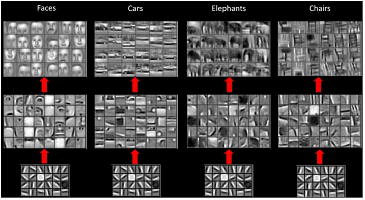
Image from this paper, based on this research

Continue in Notebook

Let's continue exploring how convolutional neural networks work, and how we can achieve trainable filters, in corresponding notebooks:

• Convolutional Neural Networks - PyTorch
• Convolutional Neural Networks - TensorFlow

Pyramid Architecture

Most of CNNs used for image processing follow so-called pyramid architecture. First convolutional layer applied to the original images typically has relatively low number of filters (8-16), which correspond to different pixel combinations, such as horizontal/vertical lines of strokes. At the next level, we reduce the spatial dimension of the network, and increase the number of filters, which corresponds to more possible combinations of simple features. With each layer, as we move towards the final classifier, spatial dimensions of the image decrease, and the number of filters grow.

As an example, let's look at the architecture of VGG-16, a network that achieved 92.7% accuracy in ImageNet top-5 classification in 2014:

Image from Researchgate

Often Used CNN Architectures

Lab

In the lab, you are tasked with classification of different cats and dogs breeds. Images are more complex than MNIST dataset and of higher dimensions, and there are more than 10 classes.

CNNs for Other Tasks

While CNNs are most often used for Computer Vision tasks, they are generally good for extracting fix-sized patterns. For example, if we are dealing with sounds, we may also want to use CNNs to look for some specific patterns in audio signal - in which case filters would be 1-dimensional (and this CNN would be called 1D-CNN). Also, sometimes 3D-CNN is used to extract features in multi-dimensional space, such as certain events occurring on video - CNN can capture certain patterns of feature changing over time.

Pre-trained Networks and Transfer Learning

Training CNNs can take a lot of time, and a lot of data is required for that task. However, much of the time is spent to learn the best low-level filters that a network is using to extract patterns from images. A natural question arises - can we use a neural network trained on one dataset and adapt it to classifying different images without full training process?

This approach is called transfer learning, because we transfer some knowledge from one neural network model to another. In transfer learning, we typically start with a pre-trained model, which has been trained on some large image dataset, such as ImageNet. Those models can already do a good job extracting different features from generic images, and in many cases just building a classifier on top of those extracted features can yield a good result.

Pre-Trained Models as Feature Extractors

Convolutional networks that we have talked about in previous section contained a number of layers, each of which is supposed to extract some features from the image, starting from low-level pixel combinations (such as horizontal/vertical line or stroke), up to higher level combinations of features, corresponding to things like an eye of a flame. If we train CNN on sufficiently large dataset of generic and diverse images, the network should learn to extract those common features.

Both Keras and PyTorch contain functions to easily load pre-trained neural network weights for some common architectures, most of which were trained on ImageNet images. The most often used ones are described in CNN Architectures page. In particular, you may want to consider using one of the following:

• VGG-16/VGG-19 are relatively simple models, but they give good accuracy. Often using VGG as a first attempt is a good choice to see how transfer learning is working.
• ResNet is a family of models proposed by Microsoft Research in 2015. They have more layers, and thus take more resources.
• MobileNet is a family of models with reduced size, suitable for mobile devices. Use them if you are short in resources, and can sacrifice a little bit of accuracy.

Here are sample features extracted from a picture of a cat by VGG-16 network:

Cats vs. Dogs Dataset

In this example, we will use a dataset of Cats and Dogs, which is very close to a real-life image classification scenario.

Continue in Notebook

Let's see transfer learning in action in corresponding notebooks:

• Transfer Learning - PyTorch
• Transfer Learning - TensorFlow

Lab

In this lab, we will use real-life Oxford-IIIT pets dataset with 35 breeds of cats and dogs, and we will build a transfer learning classifier.

Autoencoders

When training CNNs, one of the problems is that we need a lot of labeled data. In the case of image classification, we need to separate images into different classes, which is a manual effort.

However, we might want to use raw (unlabeled) data for training CNN feature extractors, which is called self-supervised learning. Instead of labels, we will use training images as both network input and output. The main idea of autoencoder is that we will have an encoder network that converts input image into some latent space (normally it is just a vector of some smaller size), the then decoder network, whose goal would be to reconstruct the original image.

Since we are training autoencoder to capture as much of the information from the original image as possible for accurate reconstruction, the network tries to find the best embedding of input images to capture the meaning.л.

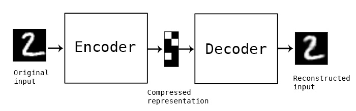
Image from Keras blog

Scenarios for using Autoencoders

While reconstructing original images does not seem useful in its own right, there are a few scenarios where autoencoders are especially useful:

• Lowering the dimension of images for visualization or training image embeddings. Usually autoencoders give better results than PCA, because it takes into account spatial nature of images and hierarchical features
• Denoising, i.e. removing noise from the image. Because noise carries out a lot of useless information, autoencoder cannot fit it all into relatively small latent space, and thus it captures only important part of the image. When training denoisers, we start with original images, and use images with artificially added noise as input for autoencoder.
• Super-resolution, increasing image resolution. We start with high-res images, and use the image with lower resolution as autoencoder input.
• Generative models. Once we train autoencoder, the decoder part can be used to create new objects starting from random latent vectors.

Variational Autoencoders (VAE)

Traditional autoencoders reduce the dimension of the input data somehow, figuring out the important features of input images. However, latent vectors ofter do not make much sense. In other words, taking MNIST dataset as an example, figuring out which digits correspond to different latent vectors is not an easy task, because close latent vectors would not necessarily correspond to the same digits.

On the other hand, to train generative models it is better to have some understanding of the latent space. This idea leads us to variational autoencoder (VAE).

VAE is the autoencoder that learns to predict statistical distribution of the latent parameters, so-called latent distribution. For example, we may want latent vectors to be distributed normally with some mean z_mean and standard deviation z_sigma (both mean and standard deviation are vectors of some dimensionality d). Encoder in VAE learns to predict those parameters, and then decoder takes a random vector from this distribution to reconstruct the object.

To summarize:

• From input vector, we predict z_mean and z_log_sigma (instead of predicting the standard deviation itself, we predict it's logarithm)
• We sample a vector sample from the distribution N(z_mean,exp(z_{log_sigma}))
• Decoder tries to decode the original image using sample as an input vector

Image from this blog post by Isaak Dykeman

Variational auto-encoders use complex loss function that consists of two parts:

• Reconstruction loss is the loss function that shows how close reconstructed image is to the target (can be MSE). It is the same loss function as in normal autoencoders.
• KL loss, which ensures that latent variable distributions stays close to normal distribution. It is based on the notion of Kullback-Leibler divergence - a metric to estimate how similar two statistical distributions are.

One important advantage of VAEs is that they allow us to generate new images relatively easy, because we know which distribution to sample latent vectors from. For example, if we train VAE with 2D latent vector on MNIST, we can then vary components of the latent vector to get different digits:

Image generated by author

Observe how images blend into each other, as we start getting latent vectors from the different portions of the latent parameter space. We can also visualize this space in 2D:

Image generated by author

Continue to Notebooks

• Autoencoders in TensorFlow

Properties of Autoencoders

• Data Specific - they only work well with the type of images they have been trained on. For example, if we train super-resolution network on flowers, it will not work well on portraits. This is because the network can produce higher resolution image by taking fine details from features learnt from the training dataset.
• Lossy - reconstructed image is not the same as the original image. The nature of loss is defined by the loss function used during training
• Works on unlabeled data

Reference

• Building Autoencoders in Keras
• Blog post on NeuroHive
• Variational Autoencoders Explained
• Conditional Variational Autoencoders

Generative Adversarial Networks

In the previous section, we have learnt about generative models - i.e. models that can generate new images similar to the ones in the training dataset. VAE was a good example of generative model.

However, if we try to generate something really meaningful, like a painting at reasonable resolution, with VAE, we will see that training does not converge well. There is another architecture specifically targeted at generative models - Generative Adversarial Networks, or GANs.

The main idea of GAN is to have two neural networks that will be trained against each other:

Image by Dmitry Soshnikov

• Generator is a network that takes some random vector, and produces the image as a result
• Discriminator is a network that takes an image, and it should tell whether it is a real image (from training dataset), or it was generated by a generator. It is essentially an image classifier.

Discriminator

The architecture of discriminator does not differ from an ordinary image classification network. In simplest case it can be fully-connected classifier, but most probably it will be a convolutional network.

GAN based on convolutional networks is called DCGAN

CNN discriminator consists of the following layers: several convolutions+poolings (with decreasing spatial size and ), one-or-more fully-connected layers to get "feature vector", final binary classifier.

Generator

Generator is slightly more tricky. You can consider it to be a reversed discriminator - starting from latent vector (in place of a feature vector), it has fully-connected layer to convert it into required size/shape, followed by deconvolutions+upscaling. This is similar to decoder part of autoencoder.

Because convolution layer is implemented as a linear filter traversing the image, deconvolution is essentially similar to convolution, and can be implemented using the same layer logic.

Image by Dmitry Soshnikov

Training the GAN

GANs are called adversarial because there is a constant competition between generator and discriminator. During this competition, both generator and discriminator improve, thus the network learns to produce better and better pictures.

The training happens in two stages:

• Training the discriminator. It is pretty straightforward: we generate a batch of images by the generator (for them label would be 0, which stands for fake image), and take a batch of images from the input dataset (with label 1, real image). We obtain some discriminator loss, and perform back prop.
• Training the generator. This is slightly more tricky, because we do not know the expected output for the generator directly. We take the whole GAN network consisting of generator followed by discriminator, feed it with some random vectors, and expect the result to be 1 (corresponding to real images). We then freeze the parameters of the discriminator (we do not want it to be trained at this step), and perform the back prop.

During this process, both generator and discriminator losses are not going down significantly. In the ideal situation, they should oscillate, corresponding to both networks improving their performance.

Go to Notebook

• GAN Notebook in TensorFlow/Keras
• GAN Notebook in PyTorch

Problems with GAN training

GANs are known to be especially difficult to train. Here are a few problems:

• Mode Collapse. By this term we mean that generator learns to produce one successful image that tricks the generator, and not a variety of different images.
• Sensitivity to hyperparameters. Often you can see that GAN does not converge at all, and then suddenly decrease in the learning rate can lead to convergence.
• Keeping balance between generator and discriminator. In many cases discriminator loss can drop to zero relatively quickly, which results in generator being unable to train further. To overcome this, we can try setting different learning rates for generator and discriminator, or skip discriminator training if the loss is already too low.
• Training for high resolution. It is the same problems as with autoencoders, because reconstructing too many layers of convolutional network leads to artifacts. This problem is typically solved with so-called progressive growing, when first a few layers are trained on low-res images, and then layers are "unblocked" or added. Another solutions would be adding extra connections between layers and training several resolutions at once - see Multi-Scale Gradient GANs paper for details.

References

• Marco Pasini, 10 Lessons I Learned Training GANs for one Year
• StyleGAN, a de facto GAN architecture to consider
• Creating Generative Art using GANs on Azure ML

Segmentation

We have already learnt about Object Detection, which allows us to locate objects in the image by predicting their bounding boxes. However, for some tasks we do not only need bounding boxes, but also more precise object localization. This task is called segmentation.

Segmentation can be viewed as pixel classification, whereas for each pixel of image we must predict its class (background being one of the classes). There are two main segmentation algorithms:

• Semantic segmentation only tells pixel class, and does not make a distinction between different objects of the same class
• Instance segmentation divides classes into different instances.

For instance segmentation 10 sheep are different objects, for semantic segmentation all sheep are represented by one class.

Image from this blog post

There are different neural architectures for segmentation, but they all have the same structure. In a way, it is similar to autoencoder, but instead of deconstructing the original image, our goal is to deconstruct a mask. Thus, segmentation network has the following parts:

• Encoder extracts features from input image
• Decoder transforms those features into the mask image, with the same size and number of channels corresponding to the number of classes.

Image from this publication

We should especially mention the loss function that is used for segmentation. In classical autoencoders we need to measure the similarity between two images, and we can use mean square error to do that. In segmentation, each pixel in the target mask image represents the class number (one-hot-encoded along the third dimension), so we need to use loss functions specific for classification - cross-entropy loss, averaged over all pixels. If the mask is binary - binary cross-entropy loss (BCE) is used.

Segmentation for Medical Imaging

In this lesson, we will see the segmentation in action by training the network to recognize human nevi on the medical images. We will be using PH² Database of dermoscopy images. This dataset contains 200 images of three classes: typical nevus, atypical nevus, and melanoma. All images also contain corresponding mask that outline the nevus.

We will train a model to segment any nevus from the background.

Notebooks

Open the notebook to learn more about different semantic segmentation architectures and see them in action.

Lab

In this lab, we encourage you to try ** human body segmentation** using Segmentation Full Body MADS Dataset from Kaggle.

Assignment

Body segmentation is just one of the common tasks that we can do with images of people. Another important tasks include skeleton detection and pose detection. Try out OpenPose library to see how pose detection can be used.

Representing Text as Tensors

Text Classification

Throughout the first part of this course, we will focus on text classification task. We will use AG News Dataset, which contains news articles like the following:

• Category: Sci/Tech
• Title: Ky. Company Wins Grant to Study Peptides (AP)
• Body: AP - A company founded by a chemistry researcher at the University of Louisville won a grant to develop...

Our goal would be to classify the news item into one of the categories based on text.

Representing text

If we want to solve Natural Language Processing (NLP) tasks with neural networks, we need some way to represent text as tensors. Computers already represent textual characters as numbers that map to fonts on your screen using encodings such as ASCII or UTF-8.

Image source

We understand what each letter represents, and how all characters come together to form the words of a sentence. However, computers by themselves do not have such an understanding, and neural network has to learn the meaning during training.

Therefore, we can use different approaches when representing text:

• Character-level representation, when we represent text by treating each character as a number. Given that we have C different characters in our text corpus, the word Hello would be represented by 5xC tensor. Each letter would correspond to a tensor column in one-hot encoding.
• Word-level representation, in which we create a vocabulary of all words in our text, and then represent words using one-hot encoding. This approach is somehow better, because each letter by itself does not have much meaning, and thus by using higher-level semantic concepts - words - we simplify the task for the neural network. However, given large dictionary size, we need to deal with high-dimensional sparse tensors.

Regardless of the representation, we first need to convert text into a sequence of tokens, one token being either a character, a word, or sometimes even part of a word. Then, we convert token into a number, typically using vocabulary, and this number can be fed into a neural network using one-hot encoding.

N-Grams

In natural language, precise meaning of words can only be determined in context. For example, meanings of neural network and fishing network are completely different. One of the ways to take this into account is to build our model on pairs of words, and considering word pairs as separate vocabulary tokens. In this way, the sentence I like to go fishing will be represented by the following sequence of tokens: I like, like to, to go, go fishing. The problem with this approach is that the dictionary size grows significantly, and combinations like go fishing and go shopping are presented by different tokens, which do not share any semantic similarity despite the same verb.

In some cases, we may consider using tri-grams -- combinations of three words -- as well. Thus the approach is such is often called n-grams. Also, it makes sense to use n-grams with character-level representation, in which case n-grams will roughly correspond to different syllabi.

Bag-of-Words and TF/IDF

When solving tasks like text classification, we need to be able to represent text by one fixed-size vector, which we will use as an input to final dense classifier. One of the simplest ways to do that is to combine all individual word representations, eg. by adding them. If we add one-hot encodings of each word, we will end up with a vector of frequencies, showing how many times each word appears inside the text. Such representation of text is called bag of words (BOW).

Image by author

BOW essentially represents which words appear in text and in which quantities, which can indeed be a good indication of what the text is about. For example, news article on politics is likely to contains words such as president and country, while scientific publication would have something like collider, discovered, etc. Thus, word frequencies can in many cases be a good indicator of text content.

The problem with BOW is that certain common words, such as and, is, etc. appear in most of the texts, and they have highest frequencies, masking out the words that are really important. We may lower the importance of those words by taking into account the frequency at which words occur in the whole document collection. This is the main idea behind TF/IDF approach, which is covered in more detail in the notebooks below.

However, none of those approaches can fully take into account the semantics of text. We need more powerful neural networks models, which we will discuss later in this course.

Continue to Notebooks

• Text Representation with PyTorch
• Text Representation with TensorFlow

Embeddings

When training classifiers based on BoW or TF/IDF, we operated on high-dimensional bag-of-words vectors with length vocab_size, and we were explicitly converting from low-dimensional positional representation vectors into sparse one-hot representation. This one-hot representation is not memory-efficient, in addition, each word is treated independently from each other, i.e. one-hot encoded vectors do not express any semantic similarity between words.

The idea of embedding is to represent words by lower-dimensional dense vectors, which somehow reflect semantic meaning of a word. We will later discuss how to build meaningful word embeddings, but for now let's just think of embeddings as a way to lower dimensionality of a word vector.

So, embedding layer would take a word as an input, and produce an output vector of specified embedding_size. In a sense, it is very similar to Linear layer, but instead of taking one-hot encoded vector, it will be able to take a word number as an input, allowing us to avoid creating large one-hot-encoded vectors.

By using embedding layer as a first layer in our classifier network, we can switch from bag-or-words to embedding bag model, where we first convert each word in our text into corresponding embedding, and then compute some aggregate function over all those embeddings, such as sum, average or max.

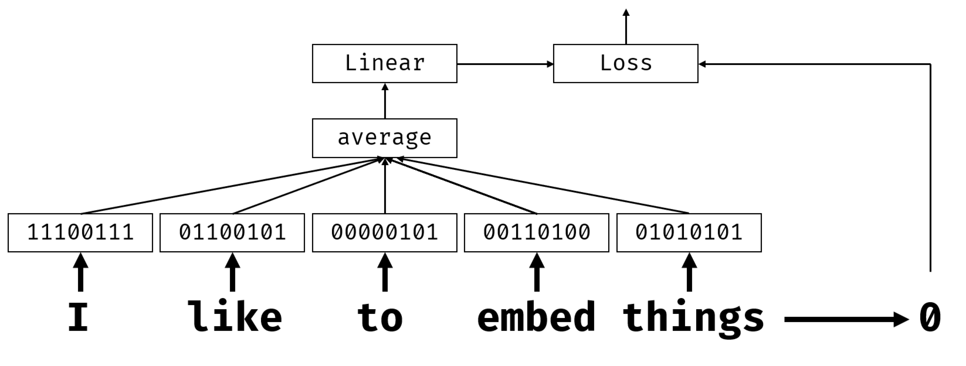
Image by author

Continue in Notebooks

• Embeddings with PyTorch
• Embeddings TensorFlow

Semantic Embeddings: Word2Vec

While embedding layer learnt to map words to vector representation, however, this representation did not necessarily have much semantical meaning. It would be nice to learn such vector representation that similar words or symonims correspond to vectors that are close to each other in terms of some vector distance (eg. Euclidean distance).

To do that, we need to pre-train our embedding model on a large collection of text in a specific way. One of the first ways to train semantic embeddings is called Word2Vec. It is based on two main architectures that are used to produce a distributed representation of words:

• Continuous bag-of-words (CBoW) — in this architecture, we train the model to predict a word from surrounding context. Given the ngram (W_{-2},W_{-1},W_0,W_1,W_2), the goal of the model is to predict W_0 from (W_{-2},W_{-1},W_1,W_2).
• Continuous skip-gram is opposite to CBoW. The model uses surrounding window of context words to predict the current word.

CBoW is faster, while skip-gram is slower, but does a better job of representing infrequent words.

Image from this paper

Word2Vec pre-trained embeddings (as well as other similar models, such as GloVe) can also be used in place of embedding layer in neural networks. However, we need to deal with vocabularies, because the vocabulary used to pre-train Word2Vec/GloVe is likely to differ from the vocabulary in our text corpus. Have a look into Notebooks to see how this problem can be resolved.

Contextual Embeddings

One key limitation of tradition pretrained embedding representations such as Word2Vec is the problem of word sense disambiguation. While pretrained embeddings can capture some of the meaning of words in context, every possible meaning of a word is encoded into the same embedding. This can cause problems in downstream models, since many words such as the word 'play' have different meanings depending on the context they are used in.

For example word 'play' in those two different sentences have quite different meaning:

• I went to a play at the theature.
• John wants to play with his friends.

The pretrained embeddings above represent both of these meanings of the word 'play' in the same embedding. To overcome this limitation, we need to build embeddings based on the language model, which is trained on a large corpus of text, and knows how words can be put together in different contexts. Discussing contextual embeddings is out of scope for this tutorial, but we will come back to them when talking about language models later in the course.

References

• Paper on Word2Vec: Efficient Estimation of Word Representations in Vector Space

Language Modeling

Semantic embeddings, such as Word2Vec and GloVe, are in fact a first step towards language modeling - creating models that somehow understand (or represent) the nature of the language.

The main idea behind language modeling is training them on unlabeled datesets in unsupervised manner. It is important, because we have huge amounts of unlabeled text available, while the amount of labeled text would always be limited by the amount of effort we can spend on labeling. Most often, we build language models that can predict missing words in the text, because it is easy to mask out a random word in text and use it as a training sample.

Training embeddings

In our previous examples, we have been using pre-trained semantic embeddings, but it is interesting to see how those embeddings can be trained using either CBoW, or Skip-gram architectures.

Image from this paper

The idea of CBoW is exactly predicting a missing word, however, to do this we take a small sliding window of text tokens (we can denote them from W_-2 to W₂), and train a model to predict the central word W₀ from few surrounding words.

More Info

• Official PyTorch tutorial on Language Modeling.
• Official TensorFlow tutorial on training Word2Vec model.
• Using gensim framework to train most commonly used embeddings in a few lines of code is as described in this documentation.

Recurrent Neural Networks

In the previous sections, we have been using rich semantic representations of text, and a simple linear classifier on top of the embeddings. What this architecture does is to capture aggregated meaning of words in a sentence, but it does not take into account the order of words, because aggregation operation on top of embeddings removed this information from the original text. Because these models are unable to model word ordering, they cannot solve more complex or ambiguous tasks such as text generation or question answering.

To capture the meaning of text sequence, we need to use another neural network architecture, which is called a recurrent neural network, or RNN. In RNN, we pass our sentence through the network one symbol at a time, and the network produces some state, which we then pass to the network again with the next symbol.

Image by author

Given the input sequence of tokens X₀,...,X_n, RNN creates a sequence of neural network blocks, and trains this sequence end-to-end using back propagation. Each network block takes a pair (X_i,S_i) as an input, and produces S_i+1 as a result. Final state S_n or (output Y_n) goes into a linear classifier to produce the result. All network blocks share the same weights, and are trained end-to-end using one backpropagation pass.

Because state vectors S₀,...,S_n are passed through the network, it is able to learn the sequential dependencies between words. For example, when the word not appears somewhere in the sequence, it can learn to negate certain elements within the state vector, resulting in negation.

Since weights of all RNN blocks on the picture are shared, the same picture can be represented as one block (on the right) with a recurrent feedback loop, which passes output state of the network back to the input.

Anatomy of RNN Cell

Let's see how simple RNN cell is organized. It accepts previous state S_i-1 and current symbol X_i as inputs, and has to produce output state S_i (and, sometimes, we are also interested in some other output Y_i, as in case with generative networks).

Simple RNN cell has two weight matrices inside: one transforms input symbol (let call it W), and another one transforms input state (H). In this case the output of the network is calculated as σ(W×X_i+H×S_i-1+b), where σ is the activation function, b is additional bias.

Image by author

In many cases, input tokens are passed through the embedding layer before entering the RNN to lower the dimensionality. In this case, if the dimension of the input vectors is emb_size, and state vector is hid_size - the size of W is emb_size×hid_size, and the size of H is hid_size×hid_size.

Long Short Term Memory (LSTM)

One of the main problems of classical RNNs is so-called vanishing gradients problem. Because RNNs are trained end-to-end in one back-propagation pass, it is having hard times propagating error to the first layers of the network, and thus the network cannot learn relationships between distant tokens. One of the ways to avoid this problem is to introduce explicit state management by using so called gates. There are two most known architectures of this kind: Long Short Term Memory (LSTM) and Gated Relay Unit (GRU).

LSTM Network is organized in a manner similar to RNN, but there are two states that are being passed from layer to layer: actual state C, and hidden vector H. At each unit, hidden vector H_i is concatenated with input X_i, and they control what happens to the state C via gates. Each gate is a neural network with sigmoid activation (output in the range [0,1]), which can be thought of as bitwise mask when multiplied by the state vector. There are the following gates (from left to right on the picture above):

• forget gate takes hidden vector and determines, which components of the vector C we need to forget, and which to pass through.
• input gate takes some information from the input and hidden vector, and inserts it into state.
• output gate transforms state via some linear layer with tanh activation, then selects some of its components using hidden vector H_i to produce new state C_i+1.

Components of the state C can be thought of as some flags that can be switched on and off. For example, when we encounter a name Alice in the sequence, we may want to assume that it refers to female character, and raise the flag in the state that we have female noun in the sentence. When we further encounter phrases and Tom, we will raise the flag that we have plural noun. Thus by manipulating state we can supposedly keep track of grammatical properties of sentence parts.

Note: A great resource for understanding internals of LSTM is this great article Understanding LSTM Networks by Christopher Olah.

Bidirectional and multilayer RNNs

We have discussed recurrent networks that operate in one direction, from beginning of a sequence to the end. It looks natural, because it resembles the way we read and listen to speech. However, since in many practical cases we have random access to the input sequence, it might make sense to run recurrent computation in both directions. Such networks are call bidirectional RNNs. When dealing with bidirectional network, we would need two hidden state vectors, one for each direction.

Recurrent network, one-directional or bidirectional, captures certain patterns within a sequence, and can store them into state vector or pass into output. As with convolutional networks, we can build another recurrent layer on top of the first one to capture higher level patterns, build from low-level patterns extracted by the first layer. This leads us to the notion of multi-layer RNN, which consists of two or more recurrent networks, where output of the previous layer is passed to the next layer as input.

Picture from this wonderful post by Fernando López

Continue to Notebooks

• RNNs with PyTorch
• RNNs with TensorFlow

RNNs for other tasks

In this unit, we have seen that RNNs can be used for sequence classification, but in fact, they can handle many more tasks, such as text generation, machine translation, and more. We will consider those tasks in the next unit.

Generative networks

Recurrent Neural Networks (RNNs) and their gated cell variants such as Long Short Term Memory Cells (LSTMs) and Gated Recurrent Units (GRUs) provided a mechanism for language modeling, i.e. they can learn word ordering and provide predictions for next word in a sequence. This allows us to use RNNs for generative tasks, such as ordinary text generation, machine translation, and even image captioning.

In RNN architecture we discussed in the previous unit, each RNN unit produced next next hidden state as an output. However, we can also add another output to each recurrent unit, which would allow us to output a sequence (which is equal in length to the original sequence). Moreover, we can use RNN units that do not accept an input at each step, and just take some initial state vector, and then produce a sequence of outputs.

This allows for different neural architectures that are shown in the picture below:

Image from blog post Unreasonable Effectiveness of Recurrent Neural Networks by Andrej Karpaty

• One-to-one is a traditional neural network with one input and one output
• One-to-many is a generative architecture that accepts one input value, and generates a sequence of output values. For example, if we want to train image captioning network that would produce a textual description of a picture, we can a picture as input, pass it through CNN to obtain hidden state, and then have recurrent chain generate caption word-by-word
• Many-to-one corresponds to RNN architectures we described in the previous unit, such as text classification
• Many-to-many, or sequence-to-sequence corresponds to tasks such as machine translation, where we have first RNN collect all information from the input sequence into the hidden state, and another RNN chain unrolls this state into the output sequence.

In this unit, we will focus on simple generative models that help us generate text. For simplicity, we will use character-level tokenization.

The way we will train RNN to generate text is the following. On each step, we will take a sequence of characters of length nchars, and ask the network to generate next output character for each input character:

When generating text (during inference), we start with some prompt, which is passed through RNN cells to generate intermediate state, and then from this state the generation starts. We generate one character at a time, and pass the state and the generated character to another RNN cell to generate the next one, until we generate enough characters.

Image by author

Continue to Notebooks

• Generative Networks with PyTorch
• Generative Networks with TensorFlow

Soft text generation and temperature

Output of each RNN cell is a probability distribution of characters. If we always take the character with highest probability as the next character in generated text, the text often can become "cycled" between the same character sequences again and again, like in this example:

today of the second the company and a second the company ...

However, if we look at the probability distribution for the next character, it could be that the difference between a few highest probabilities is not huge, e.g. one character can have probability 0.2, another - 0.19, etc. For example, when looking for the next character in the sequence 'play', next character can equally well be either space, or e (as in the word player).

This leads us to the conclusion that it is not always "fair" to select the character with higher probability, because choosing the second highest might still lead us to meaningful text. It is more wise to sample characters from the probability distribution given by the network output. We can also use a parameter, temperature, that will flatten out the probability distribution, in case we want to add more randomness, or make it more steep, if we want to stick more to the highest-probability characters.

Have a look at how this soft text generation is implemented in the notebooks.

Attention mechanisms and transformers

One of the most important problems in NLP domain is machine translation. In this section, we will focus on machine translation, or, more generally, on any sequence-to-sequence task (which is also called sentence transduction).

With RNNs, sequence-to-sequence is implemented by two recurrent networks, where one network (encoder) collapses input sequence into hidden state, and another one, decoder, unrolls this hidden state into translated result. There are a couple of problems with this approach:

• Final state of the encoder network would have hard time remembering the beginning of a sentence, thus causing poor quality of the model on long sentences
• All words in a sequence have the same impact on the result. In reality specific words in the input sequence often have more impact on sequential outputs than others.

Attention Mechanisms provide means of weighting the contextual impact of each input vector on each output prediction of the RNN. The way it is implemented is by creating shortcuts between intermediate states of the input RNN, and output RNN. In this manner, when generating output symbol y_t, we will take into account all input hidden states h_i, with different weight coefficients α_t,i.

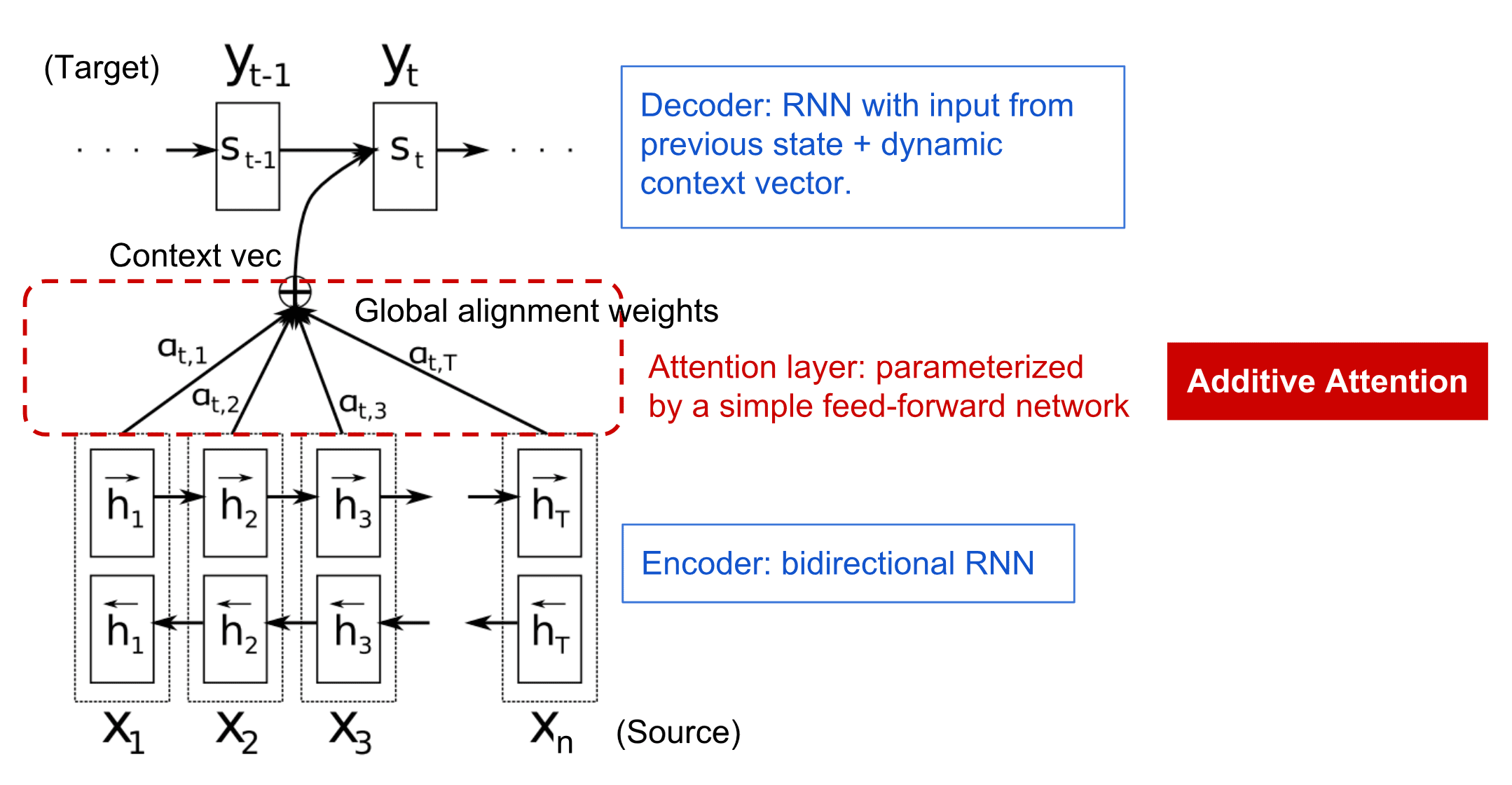
The encoder-decoder model with additive attention mechanism in Bahdanau et al., 2015, cited from this blog post

Attention matrix {α_i,j} would represent the degree which certain input words play in generation of a given word in the output sequence. Below is the example of such a matrix:

Figure from Bahdanau et al., 2015 (Fig.3)

Attention mechanisms are responsible for much of the current or near current state of the art in Natural language processing. Adding attention however greatly increases the number of model parameters which led to scaling issues with RNNs. A key constraint of scaling RNNs is that the recurrent nature of the models makes it challenging to batch and parallelize training. In an RNN each element of a sequence needs to be processed in sequential order which means it cannot be easily parallelized.

Figure from Google Blog

Adoption of attention mechanisms combined with this constraint led to the creation of the now State of the Art Transformer Models that we know and use today from BERT to Open-GPT3.

Transformer models

One of the main ideas behind transformers is to avoid sequential nature of RNNs, and create a model that is parallelizable during training. This is achieved by implementing two ideas:

• positional encoding
• using self-attention mechanism to capture patterns instead of RNNs (or CNNs) (that is why the paper that introduces transformers is called *Attention is all you need)

Positional Encoding/Embedding

The idea of positional encoding is the following. When using RNNs, the relative position of the tokens is represented by the number of step, and thus does not need to be explicitly represented. However, once we switch to attention, we need to know the relative positions of tokens within a sequence. To get positional encoding, we augment our sequence of tokens with a sequence of token positions in the sequence (i.e., a sequence of numbers 0,1, ...).

We then mix the token position with token embedding vector. To transform position (integer) into a vector, we can use different approaches:

• Trainable embedding, similar to token embedding. This is the approach we consider here. We apply embedding layers on top of both tokens and their positions, resulting in embedding vectors of the same dimensions, which we then add together.
• Fixed position encoding function, as proposed in the original paper.

Image by author

The result we get with positional embedding embeds both original token and its position within sequence.

Multi-Head Self-attention

Next, we need to capture some patterns within our sequence. To do this, transformers use self-attention mechanism, which is essentially attention applied to the same sequence as input and output. Applying self-attention allows us to take into account context within the sentence, and see which words are inter-related. For example, it allows us to see which words are referred to by coreferences, such as it, and also take the context into account:

Image from the Google Blog

In transformers, we use Multi-Head Attention, in order to give network the power to capture several different types of dependencies, eg. long-term vs. short-term word relations, co-reference vs. something else, etc.

TensorFlow Notebook contains more detains on the implementation of transformer layers.

Encoder-Decoder Attention

In transformers, attention is used in two places:

• To capture patterns within the input text using self-attention
• To perform sequence translation - it is the attention layer between encoder and decoder.

Encoder-decoder attention is very similar to the attention mechanism used in RNNs, as described in the beginning of this section. This animated diagram explains the role of encoder-decoder attention.

Since each input position is mapped independently to each output position, transformers can parallelize better than RNNs, which enables much larger and more expressive language models. Each attention head can be used to learn different relationships between words that improves downstream Natural Language Processing tasks.

BERT

BERT (Bidirectional Encoder Representations from Transformers) is a very large multi layer transformer network with 12 layers for BERT-base, and 24 for BERT-large. The model is first pre-trained on large corpus of text data (WikiPedia + books) using unsupervised training (predicting masked words in a sentence). During pre-training the model absorbs significant level of language understanding which can then be leveraged with other datasets using fine tuning. This process is called transfer learning.

Image source

There are many variations of Transformer architectures including BERT, DistilBERT. BigBird, OpenGPT3 and more that can be fine tuned. The HuggingFace package provides repository for training many of these architectures with both PyTorch and TensorFlow.

Continue to Notebooks

• Transformers in PyTorch
• Transformers in TensorFlow

Related materials

• Blog post, explaining the classical Attention is all you need paper on transformers
• A series of blog posts on transformers, explaining the architecture in detail.

Genetic Algorithms

Genetic Algorithms (GA) are based on evolutionary approach to AI, in which methods of evolution of population is used to obtain an optimal solution for a given problem. They were proposed in 1975 by John Henry Holland.

Genetic Algorithms are based on the following ideas:

• Valid solutions to the problem can be represented as genes
• Crossover allows us to combine two solutions together to obtain new valid solution
• Selection is used to select more optimal solutions using some fitness function
• Mutations are introduced to destabilize optimization and get us out of the local minimum

If you want to implement a Genetic Algorithm, you need the following:

• To find a method of coding our problem solutions using genes g∈Γ
• On the set of genes Γ we need to define fitness function fit: Γ→R. Smaller function values correspond to better solutions.
• To define crossover mechanism to combine two genes together to get a new valid solution crossover: Γ^2→Γ.
• To define mutation mechanism mutate: Γ→Γ. In many cases, crossover and mutation are quite simple algorithms to manipulate genes as numeric sequences or bit vectors.

Specific implementation of a genetic algorithm can vary from case to case, but overall structure is the following:

1. Select initial population G⊂Γ
2. Randomly select one of the operations that will be performed at this step: crossover or mutation
3. Crossover:

• Randomly select two genes g₁, g₂ ∈ G
• Compute crossover g=crossover(g₁,g₂)
• If fit(g)<fit(g₁) or fit(g)<fit(g₂) - replace corresponding gene in the population by g.

4. Mutation - select random gene g∈G and replace it by mutate(g)
5. Repeat from step 2, until we get sufficiently small value of fit, or until the limit on the number of steps is reached.

Typical Tasks

Tasks typically solved by GA:

1. Schedule optimization
2. Optimal packing
3. Optimal cutting
4. Speeding up exhaustive search

Notebooks

Go to Genetic.ipynb notebooks to see two examples of using Genetic Algorithms:

1. Fair division of treasure
2. 8 Queen Problem

Assignment

Your goal is to solve so-called Diophantine equation - an equation with integer roots. For example, consider the equation a+2b+3c+4d=30. You need to find integer roots that satisfy this equation.

Hints:

1. You can consider roots to be in the interval [0;30]
2. As a gene, consider using the list of root values

Use Diophantine.ipynb as a starting point.

This assignment is inspired by this post.

Multiagent Systems

One of the possible ways of achieving intelligence is so-called emergent (or synergetic) approach, which is based on the fact that combined behavior of many relatively simple agents can result in the overall more complex (or intelligent) behavior of the system as a whole. Theoretically, this is based on the principles of Collective Intelligence, Emergentism and Evolutionary Cybernetics, which state that higher-level systems gain some sort of added value when being properly combined from lower-level systems (so-called principle of metasystem transition).

The direction of Multi-Agent Systems has emerged in AI in 1990s as a response to growth of Internet and distributed systems. On of the classical AI textbooks, Artificial Intelligence: A Modern Approach, focuses on the view of classical AI from the point of view of Multi-agent systems.

Central to Multi-agent approach is the notion of Agent - an entity that lives in some environment, which it can perceive, and act upon. This is a very broad definition, and there could be many different types and classifications of agents:

• By their ability to reason:
  • Reactive agents usually have simple request-response type of behavior
  • Deliberative agents employ some sort of logical reasoning and/or planning capabilities
• By the place where agent execute its code:
  • Static agents work on a dedicated network node
  • Mobile agents can move their code between network nodes
• By their behavior:
  • Passive agents do not have specific goals. Such agents can react to external stimuli, but will not initiate any actions themselves.
  • Active agents have some goals which they pursue
  • Cognitive agents involve complex planning and reasoning

Multi-agent systems are nowadays used in a number of applications:

• In games, many non-player characters employ some sort of AI, and can be considered to be intelligent agents
• In video production, rendering complex 3D scenes that involve crowds is typically done using multi-agent simulation
• In systems modeling, multi-agent approach is used to simulate the behavior of a complex model. For example, multi-agent approach has been successfully used to predict the spread of COVID-19 disease worldwide. Similar approach can be used to model traffic in the city, and see how it reacts to changes in traffic rules.
• In complex automation systems, each device can act as an independent agent, which makes the whole system less monolith and more robust.

We will not spend a lot of time going deep into multi-agent systems, but consider one example of Multi-Agent Modeling.

NetLogo

NetLogo is a multi-agent modeling environment based on modified Logo programming language. This language was developed for teaching programming concepts to kids, and it allows you to control an agent called turtle, which can move, leaving a trace behind. This allows creating complex geometric figures, which is a very visual way to understand the behavior of an agent.

In NetLogo, we can create many turtles by using the create-turtles command. We can then command all turtles to do some actions (in the example below - more 10 point forward):

create-turtles 10
ask turtles [
  forward 10
]

Of course, it is not interesting when all turtles do the same thing, so we can ask groups of turtles, eg. those who are in vicinity of a certain point. We can also create turtles of different breeds using breed [cats cat] command. Here cat is the name of a breed, and we need to specify both singular and plural word, because different commands use different forms for clarity.

We will not go into learning NetLogo language - you can visit brilliant Beginner's Interactive NetLogo Dictionary resource if you are interested to learn more.

You can download and install NetLogo to try it.

Model's Library

A great thing about NetLogo is that it contains a great library of working models that you can try. Go to File → Models Library, and you have many categories of models to chose from.

You can open one of the models, for example Biology → Flocking.

Main Principles

After opening the model, you are taken to the main NetLogo screen. Here is a sample model that describes the population of wolves and sheep, given finite resources (grass).

On this screen, you can see:

• Interface section, which contains:
  • Main field, where all agents live
  • Different controls: buttons, sliders, etc.
  • Graphs that you can use to display parameters of the simulation
• Code tab contains the editor, where you can type NetLogo program

In most cases, interface would have Setup button, which initializes the simulation state, and Go button that starts execution. Those are handled by corresponding handlers in the code that look like this:

to go [
...
]

NetLogo world consist of the following objects:

• Agents (turtles) that can move across the field and do something. You command agents by using ask turtles [...] syntax, and the code in brackets is executed by all agents in turtle mode.
• Patches are square areas of the field, on which agents live. You can refer to all agents on the same patch, or you can change patch colors and some other properties. You can also ask patches to do something.
• Observer is a unique one agent that controls the world. All button handlers are executed in observer mode.

The beauty of multi-agent environment is that the code that runs in turtle mode or in patch mode is executed at the same time by all agents in parallel. Thus, by writing a little code and programming the behavior of individual agent, you can create complex behavior of the simulation system as a whole.

Flocking

As an example of multi-agent behavior, let's consider Flocking - a complex pattern that is very similar to how flocks of birds fly. Watching them fly you can think that they follow some kind of collective algorithm, or that they possess some form of collective intelligence. However, this complex behavior arises when each individual agent (bird)only observes some other agents in a short distance from it, and follows three simple rules:

• Alignment - it steers towards the average heading of neighboring agents
• Cohesion - it tries to steer towards the average position of neighbors (long range attraction)
• Separation - when getting too close to other birds, it tries to move away (short range repulsion)

You can run flocking example and observe the behavior. You can also adjust parameters, such as degree of separation, or the viewing range, which defines how far each bird can see. Note that if you decrease viewing range to 0, all birds become blind, and flocking stops. If you decrease separation to 0, all birds gather into a straight line.

Try to switch to Code tab and see where three rules of flocking (alignment, cohesion and separation) are implemented in code. Note how we refer only to those agents that are in sight.

Other Models to see

There are a few interesting models that I encourage you to experiment with:

• Art → Fireworks shows how a firework can be considered a collective behavior of individual fire streams
• Social Science → Traffic Basic and Social Science → Traffic Grid show the model of city traffic in 1D and 2D Grid with or without traffic lights. Each car in the simulation follows the simple rules:
  • If the space in front of it is empty - accelerate (up to a certain max speed)
  • If it sees the obstacle in front - brake (and you can adjust how far a driver can see)
• Social Science → Party shows how people group together during a cocktail party. You can find the combination of parameters that lead to the fastest increase of happiness of the group.

As you can see from those examples, multi-agent simulations can be quite a useful way to understand the behavior of a complex system consisting of individuals that follow the same or similar logic. It can also be used to control virtual agents, such as NPCs in computer games, or agents in 3D animated worlds.

Deliberative Agents

Agents above were typically very simple, reacting to changes in environment using some kind of algorithm - reactive agents. However, sometimes agents can reason and plan their action, in which case they are called deliberative.

A typical example would be a personal agent that receives an instructions from human to book a vacation tour. Suppose that there are many agents that live on the internet, who can help it. It should then contact other agents to see which flights are available, what are the hotel prices for different dates, and try to negotiate the best price. When the vacation plan is complete and confirmed by the owner, it can proceed with booking.

In order to do that, agents need to communicate. And for successful communication they need:

• Some standard languages to exchange knowledge, such as Knowledge Interchange Format (KIF) and Knowledge Query and Manipulation Language (KQML). Those languages are designed based on Speech Act theory.
• Those languages should also include some protocols for negotiations, based on different auction types.
• A common ontology to use, so that they refer to the same concepts knowing their semantics
• A way to discover what different agents can do, also based on some sort of ontology

Deliberative agents are much more complex than reactive, because they do not only react to changes in environment, they should also be able to intiate actions. One of the proposed architectures for deliberative agents is so-called Belief-Desire-Intention (BDI):

• Beliefs form a set of knowledge about environment that the agent has. It can be structures as knowledgebase or set of rules that an agent can apply to a specific situation in the environment.
• Desires define what agents wants to do, i.e. its goals. For example, the goal of the personal assistant agent above is to book a tour, and the goal of hotel agent is to maximize profit.
• Intentions are specific actions that agent plans to achieve its goals. Actions typically change the environment and cause communication with other agents.

There are some platforms available for building multi-agent systems, such as JADE. This paper contains fairly recent review of multi-agent platforms, together with brief history of multi-agent systems the their different usage scenarios.

Takeaway

Multi-Agent systems can take very different forms and be used in many different applications. One common thing between them is focusing on simpler behavior of an individual agent, and achieving more complex behavior of the overall system due to synergetic effect.

Ethical and Responsible AI

You have almost finished this course, and I hope that by now you clearly see that AI is based on a number of formal mathematical methods that allow us to find relationships in data and train models to replicate the human behavior in some areas. At this point in history, we consider AI to be a very powerful tool to extract patterns from data, and to apply those patterns to solve new problems.

However, in science fiction we often see stories where AI presents a danger to the humankind. Usually those stories are centered around some sort of AI rebellion, when AI decides to confront human beings. This implies that AI has some sort of emotions, or can take decisions unforeseen by its developers.

The kind of AI that we have learnt about in this course is nothing more than large matrix arithmetics. It is a very powerful tool to help us solve our problems, and as any other powerful tool - it can be used for good and for bad purposes. What's also important, it can be misused.

Principles of Responsible AI

To avoid this accidental misuse of AI, Microsoft states important Principles of Responsible AI.

• Fairness is related to the important problem of model biases, which can be caused by using biased data for training. For example, when we try to predict the probability of getting a software developer job for a person, the model is likely to give higher preference to males - just because the training dataset was likely biased towards male audience. We need to carefully balance training data and investigate the model to avoid biases, and make sure that the model takes into account more relevant features.
• Reliability and Safety. By their nature, AI models can make mistakes. A neural network returns probabilities, and we need to take it into account when making decisions. Every model has some precision and recall, and we need to understand that to prevent harm that a wrong advice can cause.
• Privacy and Security have some AI-specific flavour. For example, when we use some data for training a model, this data becomes somehow "integrated" into the model. On one hand, that increases security and privacy, on the other - we need to remember which data the model was trained on.
• Inclusiveness means that we are not building AI to replace people, but rather to augment people and make our work more creative. It is also related to fairness, because when dealing with underrepresented communities, most of the datasets we collect are likely to be biased, and we need to make sure that those communities are included and correctly handled by AI.
• Transparency. This includes making sure that we are always clear about AI being used. Also, wherever possible, we want to use AI systems that are interpretable.
• Accountability. When AI models come up with some decisions, it is not always clear who is responsible for those decisions. We need to make sure that we understand the responsibility of AI decisions. In most of the cases we would want to include human being into the loop of taking important decisions, and people are made accountable.

Tools for Responsible AI

At Microsoft, we have developed Responsible AI Toolbox, which contains a set of tools:

• Interpretability Dashboard (InterpretML)
• Fairness Dashboard (FairLearn)
• Error Analysis Dashboard
• Responsible AI Dashboard that includes
  • EconML - tool for Causal Analysis, which focuses on what-if questions
  • DiCE - tool for Counterfactual Analysis allows you to see which features need to be changed to affect the decision of the model

Model Interpretability

• Glass box models
• Black box models

Model Fairness